- Published on
Devanagari Script Recognition- Comparing CNN, SVM, ViT, and Capsule Networks
- Authors

- Name
- Astik Dahal
Ever wondered how technology reads complex scripts like Devanagari? With the rise of machine learning, we can now train models to recognize these characters with incredible accuracy. In this post, we'll dive into a project that compares four powerful machine learning approaches: Convolutional Neural Networks (CNN), Support Vector Machines (SVM), Vision Transformers (ViT), and Capsule Networks (CapsNet). Spoiler: the results are impressive and actionable!
Lets explore how these models work, their strengths and weaknesses, and which one emerges as the ultimate champion in Devanagari script recognition.
The Problem
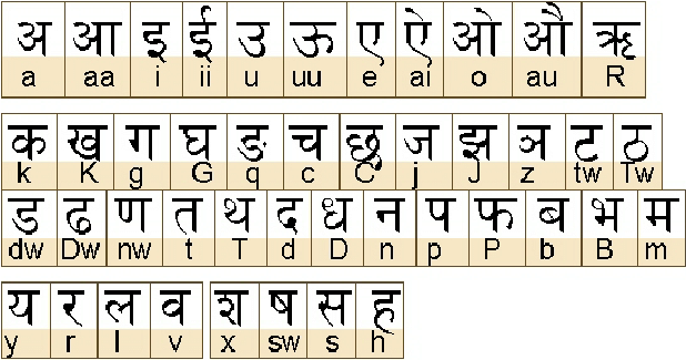
Devanagari script, used in languages like Hindi and Marathi, contains 46 unique characters. Manually processing and recognizing such characters is daunting, especially in large datasets. The objective? Develop and compare machine learning models to automate recognition with high accuracy and efficiency.
Fig: Devanagari Scripts
Our Approach
We tackled this problem using four diverse models:
- CNN: A gold standard for image recognition tasks.
- SVM: A classical algorithm with dimensionality reduction via PCA.
- ViT: A cutting-edge model leveraging transformer architecture for vision tasks.
- CapsNet: A novel approach addressing spatial hierarchies in images.
Each model was trained and tested on a dataset of grayscale images (32x32) of Devanagari characters, ensuring a fair comparison.
Explaining the Code
1. Dataset Preparation
We used a Kaggle dataset of 92,000 labeled images. After preprocessing, the data was split into training and testing sets:
from sklearn.model_selection import train_test_split
from sklearn.preprocessing import LabelEncoder

# Label encoding and splitting
label_encoder = LabelEncoder()
df['character'] = label_encoder.fit_transform(df['character'])
X_train, X_test, y_train, y_test = train_test_split(
    X, y, test_size=0.2, random_state=42
)
2. Model Architectures
CNN
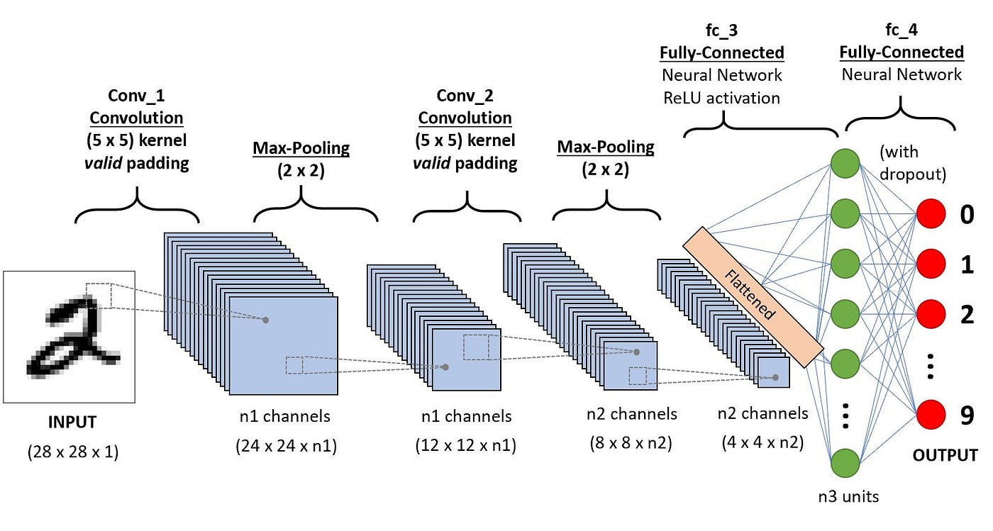
A Convolutional Neural Network (CNN) is a type of deep learning algorithm that is particularly well-suited for image recognition and processing tasks. CNNs excel at extracting spatial features.
Fig: CNN Architecture
Here’s a snippet of the architecture:
from tensorflow.keras import layers, models

cnn_model = models.Sequential([
    layers.Conv2D(64, (3,3), activation='relu', input_shape=(32,32,1)),
    layers.MaxPooling2D(),
    layers.Flatten(),
    layers.Dense(256, activation='relu'),
    layers.Dense(46, activation='softmax')
])
SVM
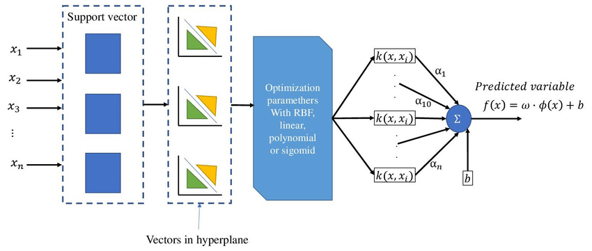
Support Vector Machines (SVM) are classical algorithms known for their robustness in smaller datasets.
Here, we used PCA for dimensionality reduction before training the SVM model:
from sklearn.decomposition import PCA
from sklearn.svm import SVC

# PCA for feature reduction
pca = PCA(n_components=100)
X_train_pca = pca.fit_transform(X_train)
X_test_pca = pca.transform(X_test)

# Training the SVM model
svm_model = SVC(kernel='rbf', C=1, gamma='scale')
svm_model.fit(X_train_pca, y_train)
ViT
ViT leverages transformers for vision tasks. Using patches and attention mechanisms, it deciphers images:
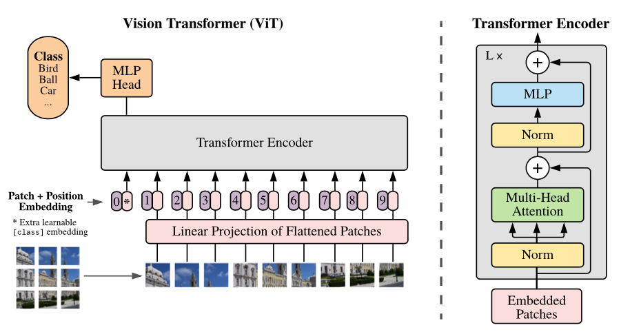
Fig: ViT Architecture
from transformers import ViTConfig, TFViTModel

config = ViTConfig(image_size=32, num_labels=46)
model_vit = TFViTModel(config)
CapsNet
Capsule Networks capture spatial hierarchies through dynamic routing.
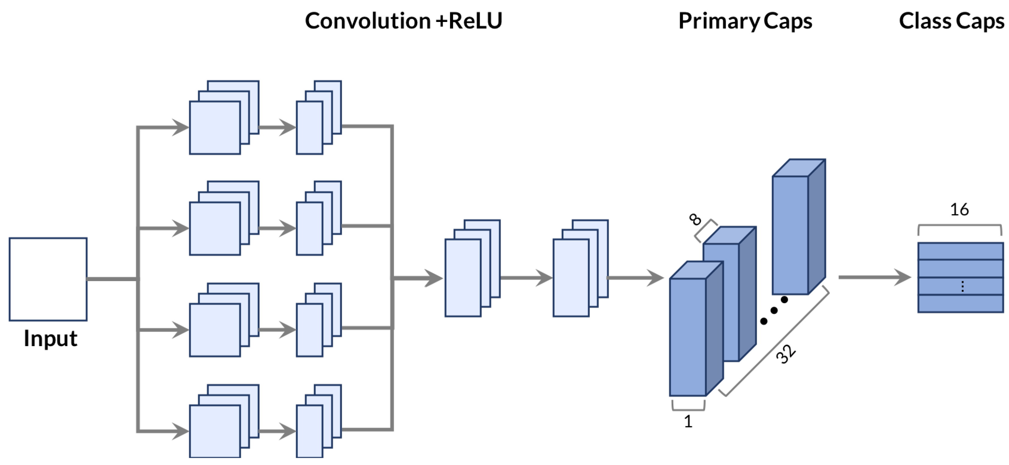
Fig: CapsNet Architecture
Here’s the implementation:
import tensorflow as tf
from tensorflow.keras import layers

# Squash function
def squash(vectors, axis=-1):
    norm = tf.norm(vectors, axis=axis, keepdims=True)
    scale = norm**2 / (1 + norm**2) / (norm + 1e-8)
    return scale * vectors

...

# Capsule Network Model
input_layer = layers.Input(shape=(32, 32, 1))
x = layers.Conv2D(64, 5, strides=1, padding='same', activation='relu')(input_layer)
x = layers.Conv2D(128, 5, strides=2, padding='same', activation='relu')(x)
primary_caps = PrimaryCaps(num_capsules=8, dim_capsule=16)(x)
digit_caps = DigitCaps(num_capsules=46, dim_capsule=16)(primary_caps)
out_caps = layers.Lambda(lambda z: tf.sqrt(tf.reduce_sum(tf.square(z), axis=2)))(digit_caps)

caps_model = tf.keras.Model(inputs=input_layer, outputs=out_caps)
caps_model.compile(optimizer='adam', loss='sparse_categorical_crossentropy', metrics=['accuracy'])
3. Epochs: Iterative Learning
An epoch represents one complete pass through the training dataset by the model. Increasing the number of epochs allows the model to learn from the data more effectively, but too many epochs can lead to overfitting.
In our project, we used 5 epochs for CNN, ViT, and CapsNet models. Here’s an example of how epochs are used in training:
# Training the CNN model
cnn_history = cnn_model.fit(
    X_train, y_train,
    validation_split=0.1,
    epochs=5,
    batch_size=32
)
This iterative process ensures the model fine-tunes its weights for better accuracy over time. The results, as seen in our performance metrics, show the importance of choosing an optimal number of epochs.
Model Performance
After training, we evaluated all models using various metrics and confusion matrices.
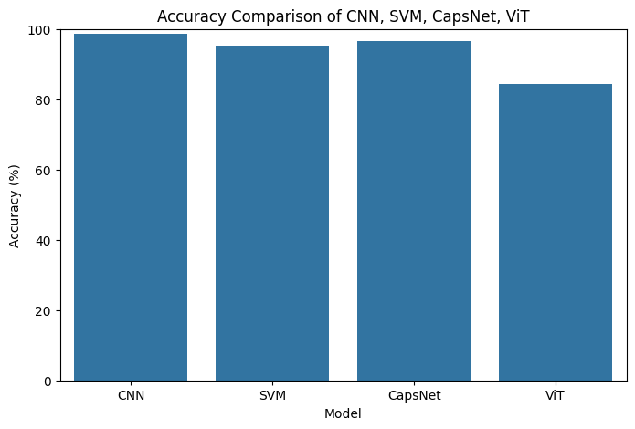
| Model | Accuracy (%) | Training Time (s) |
|---|---|---|
| CNN | 98.60 | 115.18 |
| SVM | 95.30 | 210.79 |
| CapsNet | 96.67 | 183.98 |
| ViT | 84.46 | 320.10 |
Testing the models
Here, we tested the models with some random images. All of the models predict the characters correctly, and the time for inference is also shown.
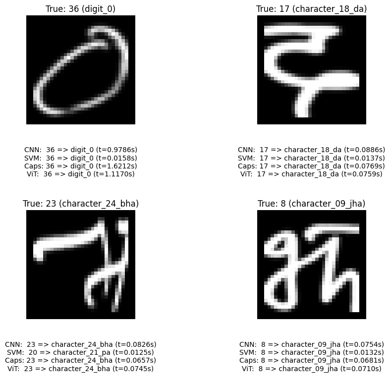
Fig: Testing of models for various characters
Classification Results Across Models
Precision, Recall, F1-Score and Support are calculated of all algorithms for devanagari script.
ViT Classification Report (First 5 sample)
| Class ID | Precision | Recall | F1-Score | Support |
|---|---|---|---|---|
| 0 | 0.93 | 0.82 | 0.87 | 380 |
| 1 | 0.70 | 0.87 | 0.78 | 404 |
| 2 | 0.92 | 0.75 | 0.82 | 371 |
| 3 | 0.77 | 0.67 | 0.72 | 404 |
| 4 | 0.83 | 0.83 | 0.83 | 423 |
| ... | ... | ... | ... | ... |
CNN Classification Report (First 5 sample)
| Class ID | Precision | Recall | F1-Score | Support |
|---|---|---|---|---|
| 0 | 1.00 | 0.99 | 0.99 | 380 |
| 1 | 1.00 | 0.99 | 1.00 | 404 |
| 2 | 1.00 | 0.99 | 0.99 | 371 |
| 3 | 0.96 | 0.98 | 0.97 | 404 |
| 4 | 0.99 | 0.97 | 0.98 | 423 |
| ... | ... | ... | ... | ... |
SVM Classification Report (First 5 sample)
| Class ID | Precision | Recall | F1-Score | Support |
|---|---|---|---|---|
| 0 | 0.99 | 0.97 | 0.98 | 380 |
| 1 | 0.94 | 0.96 | 0.95 | 404 |
| 2 | 0.97 | 0.95 | 0.96 | 371 |
| 3 | 0.91 | 0.91 | 0.91 | 404 |
| 4 | 0.94 | 0.91 | 0.93 | 423 |
| ... | ... | ... | ... | ... |
Capsule Network Classification Report (First 5 sample)
| Class ID | Precision | Recall | F1-Score | Support |
|---|---|---|---|---|
| 0 | 0.94 | 0.99 | 0.96 | 380 |
| 1 | 0.98 | 0.97 | 0.98 | 404 |
| 2 | 0.99 | 0.97 | 0.98 | 371 |
| 3 | 0.88 | 0.96 | 0.92 | 404 |
| 4 | 0.99 | 0.96 | 0.97 | 423 |
| ... | ... | ... | ... | ... |
Key Metrics
- CNN outperformed all models with a remarkable accuracy of 98.6%.
- SVM, while slower, still achieved high accuracy.
- CapsNet performed well, particularly for preserving spatial hierarchies.
- ViT lagged due to its transformer-specific requirements for larger image sizes.
Visualizations
Confusion Matrix: Below is the confusion matrix for CNN, highlighting its strong performance across all classes.
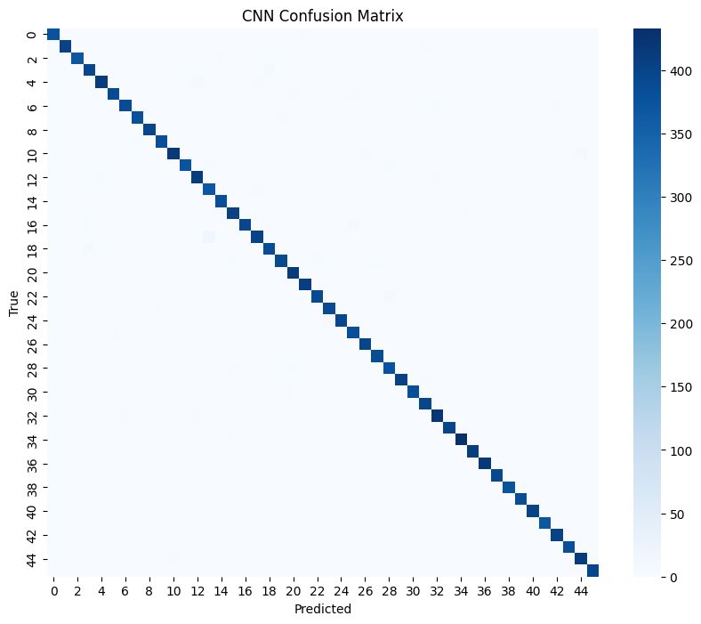
Fig: Confusion Matrix showing CNN’s prediction accuracy.

Fig: Confusion matrices of ViT, CapsNet and SVM
Takeaways and Applications
- Practical Usage: Use CNNs for fast and accurate recognition of Devanagari scripts in real-time applications like OCR tools.
- Trade-offs: For resource-constrained environments, SVM can be a viable option despite longer training times.
- Emerging Tech: CapsNet holds promise for scenarios requiring detailed spatial information, such as medical imaging.
- Future of ViT: While ViT underperformed here, its potential shines with larger datasets and higher-resolution images.
Conclusion
This project highlights the power and versatility of machine learning in solving complex problems like script recognition. By comparing CNN, SVM, ViT, and CapsNet, we’ve demonstrated that CNNs are the top choice for this task but the landscape is ever-evolving.
The code is available on google colab
